A Gun and a Radio
Link to the accompanying dashboard for visual learning! - Streamlit App

James Bond: A gun and a radio. It's not exactly Christmas, is it?
Q: Were you expecting an exploding pen? We don't really go in for that anymore.
Most cybersecurity professionals are still looking for exploding pens. They think machine learning is about finding the fanciest algorithm, but effectiveness lies in something much simpler.
This essay is for security professionals who want to understand why their machine learning models work in demos but fail in production. Feature selection, not algorithms, determines whether intrusion detection systems catch real attacks or waste analysts' time chasing false positives.
The Problem Nobody Talks About
To understand why feature selection matters more than algorithms, I built an interactive analysis using the UNSW-NB15 dataset (link here), which is one of the most widely used datasets for network intrusion detection research. This dataset gives you 49 features describing network flows: TCP flags, packet sizes, flow durations, protocol types. All the usual suspects that security engineers think matter.
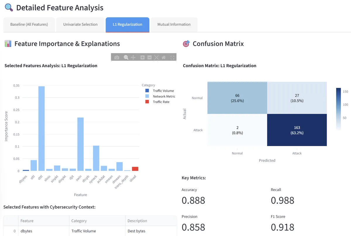
But here's what becomes clear when you actually analyze the data: in the real world, more data isn't always better data. Sometimes it's just more ways to be wrong. Most of these 49 features are noise and in order to see for yourself, go to the dashboard and run the models, excluding RFE, on 0.5% of the data and switch to the live training tab (then you can proceed to explore which features were selected by each specific algorithm, you can also select the number of features for certain methods)!
Think about it from an attacker's perspective. If you're trying to evade detection, you're not going to mess with fundamental network properties that are hard to manipulate. You'll focus on what you can control. Meanwhile, the intrusion detection system is busy learning patterns from features that change randomly between different network environments.
Welcome to the feature selection problem, and it's the difference between AI systems that work in demos and ones that work in production.
Important note on dashboard usage:
For sane training times on the free cloud, use 0.5% of the dataset without RFE selected, then switch to the live training tab to see the complete results. You can increase the percentage of data and select RFE but keep in mind that the compute power of this hosting service is very poor.
On the left hand side, you can change the training data size and select number of features for configurable methods. In the center, you have two tabs - Pre-Configured Results and Live Training. After you live train, you can access even more visualizations in the "Detailed Feature Analysis" section. This section is only available on live data!
What Goes Wrong
There are three patterns in how cybersecurity teams handle features, and two of them are disasters.
Pattern 1: Use Everything
Aka, the lazy approach. Throw all your features at XGBoost and call it a day.
But, what is the actual problem with training your model on all the features available to you? The crucial problem is that models memorize irrelevant correlations. They learn that attacks tend to happen when feature 14 has a certain value, not because feature 14 matters, but because it happened to correlate with attacks in the training set. When deploying this model in a real world scenario, feature 14 inadvertently behaves differently, and accuracy pummels depending on how much that particular feature was prioritized.
Training time also explodes. More features mean higher-dimensional spaces, which mean exponentially more computation. Models that could've taken a few seconds to train now take hours. In a dynamic SOC-type environment, where retraining on new attack patterns is constant, this kills operational tempo.
Pattern 2: Intuition-Based Selection
Aka, the dangerous approach. A security engineer looks at the feature list and picks what "makes sense." Protocol type, packet size, flow duration. The obvious stuff.
To understand why this might backfire spectacularly, let us take an example of the UNSW-NB15 dataset. A security expert would naturally gravitate toward features like 'proto' (protocol) and 'service' because they seem intuitively important. They would likely skip 'ct_srv_dst' (count of connections to same destination port) because it obviously is not as important as the protocol and service! But in the actual data, 'ct_srv_dst' turns out to be one of the most predictive features for certain attack types, while 'proto' adds little signal once you have other network flow information.
Humans are bad at this because our intuition about high-dimensional data is terrible. We think in three dimensions. Machine learning operates in higher dimensional space, which we cannot intuit our way out of.
Speaking from personal experience, my team and I spent months on our bachelor's project building a hybrid intrusion detection system, only to watch our model work perfectly on paper but fail in the real world. Our mistake? We had chosen the "obviously important features" while discarding others to improve training time.
Pattern 3: Systematic Selection
The approach that works. Let the data tell you what matters.
How to Do It Right
Real feature selection is about measuring what actually improves a model's ability to distinguish between normal traffic and attacks (or classification of any kind for that matter).
I'll be discussing 4 methods that help select the ideal features for training :
- Univariate Methods (F-test/ANOVA, Chi-square)
- Recursive Feature Elimination
- Mutual Information
- L-1 Regularization
Univariate Methods
For each feature, ask one question: "Are the values for this feature different between attacks and normal traffic?"
The key insight: Univariate selection treats every feature in isolation. It asks: "Does this single feature help distinguish attacks from normal traffic?"
Use statistical tests. For each feature, measure how much it differs between attack and normal traffic. Chi-square for categories, ANOVA for continuous data.
Example: Normal users browse randomly. Sometimes they load a 500-byte text page, sometimes a 5MB video. Attackers exfiltrating data are systematic. They grab 64KB chunks to stay under detection thresholds. ANOVA's F-test catches this because normal users vary wildly but attackers are consistent.
The ratio of "how different the groups are" to "how much each group varies internally" gives you a strong signal for detecting abnormalities.
The limitation is this only works for obvious patterns. Smart attackers randomize traffic using jitters etc. to look normal.
For categories, chi-square compares distributions. Normal users spend 70% of connections on HTTP, 20% on email, 10% on other protocols. Reconnaissance attackers look different: 10% HTTP, 15% SSH, 25% Telnet, 30% SNMP. Completely different fingerprint.
Here the limitation is that targeted attackers hitting one service slip through because their distribution looks normal enough.
In the UNSW dataset, features like 'service' and 'sttl' (source to destination time to live) typically show strong univariate relationships with attack labels. Features like 'dwin' (destination TCP window advertisement) often don't. This doesn't mean 'dwin' is useless. It might be crucial in combination with other features. But it means it's not carrying obvious signal by itself.
Even if you can see improved training times, as discussed below, there are much better methods to select fewer number of correct features.
Recursive Feature Elimination
Train a model with all features, then systematically remove the least important ones. Retrain. Measure performance. Remove more. Repeat until performance starts dropping.
Imagine you're a chef trying to perfect a recipe. You start with 20 ingredients, make the dish, and taste it. Then you remove the ingredient that seems to contribute least to the flavor, cook again, and taste again. Keep going until removing anything makes the dish noticeably worse. That's RFE.
The tricky part is measuring "contribution." For linear models, it's simple: bigger weights mean more importance, like stronger flavors dominating a dish. For tree models, importance means "how much does this ingredient help me make decisions?" If knowing whether something contains salt helps you correctly categorize 1000 dishes, but knowing the exact temperature helps with only 10 dishes, salt is more important.
The key insight is that ingredients (features) work together in unexpected ways. Removing salt might not hurt your pasta much, but removing both salt and garlic together ruins everything. Features have similar interactions.
This is computationally very expensive but reveals something crucial: which features the model actually uses. Often, 80% of performance comes from 20% of features.
You can look at the abnormal training time below as compared to other models while using only 0.5% of the data. There is a silver lining here though, the training time does not scale linearly or worse when the amount of data is large. The training time is largely dependent on the number of features.
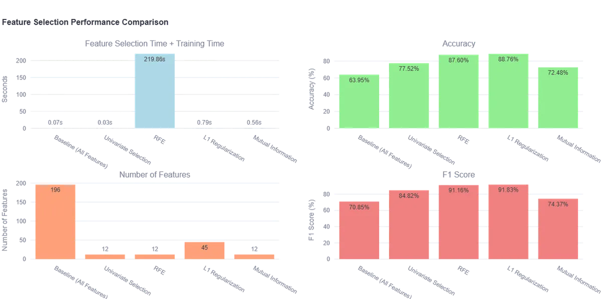
While using 0.5% of the dataset, the feature selection time + training time is observed to be 219.86 seconds, while using 20% of the dataset, this time does not jump 40X, instead we can observe it to be only 743.27 seconds.
Once the crucial features have been identified, training the model will be rather quick because of the low number of features. In the dashboard, you can even change the number of features you want the model to tune for and check accuracy!
Mutual Information
Some features are useless alone but powerful in combination. Traditional correlation measures miss these relationships. Mutual information doesn't. Here's how it works: you calculate MI(feature, target) for every feature. High MI means "knowing this feature tells me a lot about whether it's an attack." Low MI means "this feature is basically random noise." Then you rank features by their MI scores and keep the top ones.
The beauty of MI is it catches weird, non-linear relationships that correlation misses. Maybe small packets AND large packets both indicate attacks, but medium packets are normal. Correlation would be near zero because the relationship isn't linear. But MI would be high because knowing packet size still reduces uncertainty about attacks.
Correlation is like asking "when X goes up, does Y go up too?" But real relationships are often more complex. Imagine you're trying to predict if someone will buy a sports car. Age alone isn't predictive (both 25-year-olds and 45-year-olds buy them). Income alone isn't either (both rich and middle-class people buy them). But the combination is highly predictive: young people with any decent income buy sports cars, older people only if they're quite wealthy.
Mutual information captures this by asking a different question: "how much does knowing X reduce my uncertainty about Y?" Mathematically, it's MI(X,Y) = ΣΣ P(x,y) log[P(x,y)/(P(x)P(y))]. This formula compares the actual joint probability P(x,y) to what we'd expect if X and Y were independent: P(x)×P(y). When they're very different, mutual information is high.
For example, in network intrusion detection, the combination of packet size and flow duration might be meaningless individually but highly predictive together.
L1 Regularization
Add a penalty term to the loss function that punishes models for using too many features. The math automatically drives feature weights toward zero unless they're truly contributing to performance.
Think of training a model like packing for a trip where every extra item costs money. You want to pack everything useful, but you also want to minimize luggage fees. L1 regularization adds a "fee" proportional to how much stuff you pack (the sum of absolute weights): Loss = Original_Loss + λ × Σ|weights|.
The λ (lambda) parameter is like the airline's fee structure. Set λ low, and you'll pack everything and then some more. Set λ high, and you'll travel with just the absolute essentials (and any higher, you will miss out on a few essentials too!). The mathematical magic happens because of how this penalty interacts with optimization. L1 creates a "diamond-shaped" constraint in weight space. When your optimization process tries to find the best weights, it has to navigate around this diamond. The diamond has sharp corners exactly on the axes, where individual weights become zero.
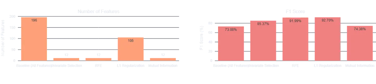
Out of the methods discussed, L1 Regularization gives the best accuracy. This, however, comes with a catch. We cannot define the number of features to be selected.
As seen below, the improvement in F1 score is rather minimal as compared to RFE (about 0.71% only). But the number of features is 10X that of RFE! This means that continuously retraining your model can be a computationally painful task. It is upto the stakeholder to perform a cost-benefit analysis and choose the right method.
Why This Matters More in Cybersecurity
Adversarial Robustness
If models rely on features that attackers can easily manipulate, you're building a system designed to fail. Good feature selection identifies the features that are fundamental to the network behavior you're trying to detect, not just correlated with it in training data.
Deployment Reality
Different operating systems, network configurations, hardware vendors create variations in features that seemed stable in training environments. Models built on correctly selected features generalize better because they're not overfitting to any particular environment.
Operational Tempo
In cybersecurity, retraining constantly as new attack patterns emerge is necessary. Feature selection usually means reduction in the total number of features which dramatically reduces training time, which means faster iteration and staying ahead of evolving threats.
The Proof
Testing different feature selection methods on the UNSW-NB15 dataset reveals the true impact of systematic feature selection. When using all available features as a baseline, proper feature selection techniques show remarkable improvements:
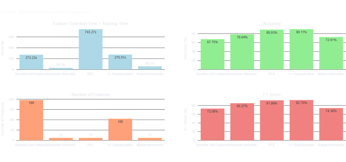
For detailed results and interactive comparisons of different feature selection methods, see the accompanying dashboard analysis.
The Bigger Picture
Feature selection reveals something fundamental about machine learning that most people miss: the goal isn't to use all available data. It's to use the right data.
This principle applies beyond cybersecurity. In any domain where detecting patterns in noisy environments matters (fraud detection, medical diagnosis, quality control), the features chosen matter as much as the algorithms used.
When feature selection is done right, everything else gets easier. Models train faster, generalize better, and break less often in production. When it's done wrong, no complicated neural network or ML model will save you.
A gun and a radio. Most of the time, that's enough.